CMUSRP 2022
Table of Contents
\( \newcommand{\contra}{\Rightarrow\!\Leftarrow} \newcommand{\R}{\mathbb{R}} \newcommand{\F}{\mathbb{F}} \newcommand{\Z}{\mathbb{Z}} \newcommand{\Zeq}{\mathbb{Z}_{\geq 0}} \newcommand{\Zg}{\mathbb{Z}_{>0}} \newcommand{\Req}{\mathbb{R}_{\geq 0}} \newcommand{\Rg}{\mathbb{R}_{>0}} \newcommand{\N}{\mathbb{N}} \newcommand{\Q}{\mathbb{Q}} \newcommand{\O}{\mathcal{O}} \newcommand{\C}{\mathbb{C}} \newcommand{\A}{\mathbb{A}} \newcommand{\P}{\mathbb{P}} \DeclareMathOperator{\Spec}{Spec} \DeclareMathOperator{\Conf}{Conf} \DeclareMathOperator{\Tot}{Tot} \DeclareMathOperator{\Fil}{Fil} \DeclareMathOperator{\Gr}{Gr} \DeclareMathOperator{\Inv}{Inv} \DeclareMathOperator{\Alt}{Alt} \DeclareMathOperator{\Sym}{Sym} \DeclareMathOperator{\Vec}{Vec} \DeclareMathOperator{\id}{id} \DeclareMathOperator{\Proj}{Proj} \DeclareMathOperator{\Func}{Func} \DeclareMathOperator{\Ker}{Ker} \DeclareMathOperator{\Im}{Im} \DeclareMathOperator{\Aut}{Aut} \DeclareMathOperator{\Ob}{Ob} \DeclareMathOperator{\Mor}{Mor} \DeclareMathOperator{\Hom}{Hom} \DeclareMathOperator{\End}{End} \DeclareMathOperator{\Ind}{Ind} \DeclareMathOperator{\Coind}{Coind} \DeclareMathOperator{\colim}{colim} \DeclareMathOperator{\length}{length} \DeclareMathOperator{\Pic}{Pic} \)
1. Introduction
1.1. Stability
Given some objects \(G_n \rightarrow G_{n+1} \rightarrow \dots\), we want to find some invariant, \(G \mapsto \text{Inv}(G)\), satisfying stability: that for sufficiently large \(n\), \(\text{Inv}(G_n) \cong \Inv(G_{n+1})\).
As an example, we can take \(\Inv(G) = G^{ab}\), the abelianization, and if for example \(G_n = GL_n(k)\), then we have stbility for \(n \geq 2\), and similar for the symplectic groups, the special linear groups, etc.
A special case we will discuss in more detail will be the symmetric groups, \(S_n\), the group of bijections from a set of \(n\) objects to itself. In particular, the abelianization sends, for \(n \geq 2\), \(S_n \mapsto \Z/2\Z\); this is appararent from the group representation \[ S_n \cong \left\langle (\sigma_i)^n_{i=1} \mid \sigma_i^2 = 1, \sigma_i\sigma_j = \sigma_i\sigma_i \text{ for } |i - j| > 2, \sigma_i\sigma_j\sigma_i = \sigma_j\sigma_i\sigma_j \text{ for } | i - j| = 1\right\rangle \] Similarly, we can look at the braid groups \(B_n\), which are given by \[ B_n \cong \left\langle (\sigma_i)^{n-1}_{i=1} \mid \sigma_i\sigma_j = \sigma_i\sigma_i \text{ for } |i - j| > 2, \sigma_i\sigma_j\sigma_i = \sigma_j\sigma_i\sigma_j \text{ for } |i - j| = 1\right\rangle \] as well as the “pure braid groups”, given by \(\Ker(B_n -> S_n)\); it is clear that the abelianization of \(B_n\) is just \(\Z\).
Furthermore, it will turn out that the abelianization of a group is the same as the first homology group, \(H_1(G)\); the second homology group will be more complication, and will be characterized by \[ H_2(G) = \frac{R \cap [F, F]}{[R, R]} \] where \(G = F/R\), and \(F\) is free.
Theorem (Nakaoka, 1960’s): For \(n \geq 2q\), \(H_q(S_n) \cong H_q(S_{n+1})\); this result was generalized to homological stability, which gives it for a lot of other sequences of groups.
A non-example will be the pure braid groups; we have already
\begin{align*} B_n &\rightarrow \Aut(P_n) \\ t &\mapsto (p \mapsto tpt^{-1}) \\ S_n &\cong B_n / P_n \rightarrow \Aut(H_q(P_n)) \end{align*}so \(H_q(P_n\) should be an abelian group with some \(S_n\)-action. More explicitly, let \(\sigma_{ij} \in B_n\) be the lift of the transposition \((i, j)\), and take \[ P_n = \left\langle (a_{ij})_{i < j} \mid [a_{ij}, -] = 1 \right\rangle \] with the map \(a_{ij} \mapsto \sigma_{ij}^2\). It also becomes clear from this representation that the abelianization of \(P_n\) will be \(\Z^{\oplus \frac{n(n-1)}{2}}\). Furthermore, we have that \[ H_1(P_n) \otimes_\Z \Q \cong \Sym^2(St_n) \] where \(St_n\) is the standard representation.
1.2. Representational Stability
This is our first example of representational stability!
In particular, we define \(\Q-\text{characters of } S_n\) to be the set of class functions of \(S_n\), or all maps to \(Q\) invariant by conjugation.
Then, we can see that \[ \chi_{St_n}(\sigma) = \chi_1(\sigma) - 1 \] and so we conclude that since \(\chi_{\Sym^2}(\sigma) = \frac{1}{2}(\chi(\sigma^2) + \chi(\sigma)^2)\), \[ \chi_{H_1(P_n)} = -\chi_2 + \binom{\chi_1}{2} \]
Theorem (Church-Farb): For \(n\) sufficiently large, \((H_q(P_n))_\Q\) is a polynomial sequence of characters of \((S_n)_n\).
1.3. FI Modules
The category \(FI\) will have objects indexed by \(m \geq 0\), with \(\Hom_{FI}(m, n)\) to be injective maps \([m] \rightarrow [n]\).
In fact, \(H_q(P_n)\) are really functions \(FI \rightarrow Ab\); \(FI\)-modules will be functors \(FI \rightarrow \Vec_\Q\); equivalently, finitely generated \(FI\)-modules will be the same as polynomial sqeuences of representations of \(S_n\).
The thing to care about is the Noetherianity of such categories. We will also consider a little bit of topology, in the sense that we may have some \(FI\)-spaces, which map \(n \mapsto \text{Conf}_n(X)\), the space of injective maps \([n] \rightarrow X\).
For example, \(\text{Conf}_n \C = \{(z_i)_{i=1}^n \mid z_i \neq z_j\}\), and the fundamental group will be \(P_n\).
Theorem (Church-Eilenberg-Farb): For \(n\) sufficiently large, then \((H_q(\text{Conf}_n(X)))_n\) is a polynomial sequence of \(G_n\)-representations.
Note that for \(n = q = 1\), we have the correspondence \[ H_1(X) = \pi_1^{ab} = H_1(\pi_1) \]
2. Categories
Definition: A category \(C\) is the data of a class \(\Ob(C)\) of objects and
- For each \(X, Y \in \Ob(C)\) a set \(\Hom_C(X,Y)\)
- For each \(X, Y, Z\) a map \(\Hom_C(X,Y) \times \Hom_C(Y,Z) \mapsto \Hom_C(X, Z)\)
- For all \(X \in \Ob(C)\), some identity element \(\id_X\) in \(\Hom_C(X,X)\)
where the morphisms satisfy associativity.
Examples:
- \(Set\)
- \(Gp\)
- For a fixed (associative, unital) ring \(R\), the category of (right) modules over \(R\), \(Mod_R\)
To be more prescise, we make the following definitions:
Definition: A morphism in \(Mod_R\) from \(M \rightarrow N\) is a group homomorphism \(f: M \rightarrow N\) satisfying that \(f(m \lambda) = f(m) \cdot \lambda\).
Example: \(R \cong \Hom_{Mod_R}(R,R)\), where \(a \mapsto (x \mapsto ax)\).
Definition Functors \(C \rightarrow D\) are a collection of data, containing
- For each \(X \in \Ob(C)\), an object \(F(X) \in \Ob(D)\)
- For each \(f \in \Hom_C(X,Y)\), some \(F(f) \in \Hom_D(F(X), F(Y))\), which satisfy
- \(F(fg) = F(f) F(g)\)
- \(F(\id_X) = \id_{F(X)}\)
We can also form now a category of categories, i.e. a 2-category, and so on onto \(n\)-categories.
OK blah blah blah a bunch of the usual category stuff that I’m not typing - adjoints, equivalences, functor categories, etc.
Example: We call the functor category \(\Func(FI, Ab)\), to be the category of \(FI\)-modules.
2.1. Finiteness Conditions
Definition: \(C\) is a small category if its objects are a set, and essentially small if it admits a small skeleton.
Definition: A subcategory \(C'\) of \(C\) is a category with objects a subclass of \(\Ob(C)\) and morphisms a subset of \(\Hom_C(\cdot, \cdot)\). It is called a full subcategory if the inclusion functor \(C' \rightarrow C\) is fully faithful, or equivalently, if \(\Hom_C' = \Hom_C\).
Definition: Finite presentation: See Stacks Project, Tag 00F3.
2.2. Limits/Colimits
Definition: Let \(I\) be a (partially) ordered set; an \(I\)-diagram on \(C\) is a functor \(F: I \rightarrow C\) when \(I\) is considered as a category; a limit of \(F\) is an object of \(C\) that represents the functor \(C \rightarrow Set\), \(X \mapsto \Hom_{\Func(I, C)}((i \mapsto X), F)\); a colimit is the same, but the \(\Hom\) arguments are reversed.
Definition A colimit is filted if \(I\) has finite supremum.
Definition An object \(X\) of \(C\) is compact if \(\Hom(X, -)\) commites with filtered colimit.
Example: In the categories of \(CRing, CAlg, Mod_R, Sets\), etc, compact is the same as finitely presented.
Proof: Let \(B\) be a compact object of \(CAlg\), and let \(I\) the category where the objects \(S \subset B\) finite sets and \(I \subset A[(x_s)]_{s \in S}\) is a finitely generalted ideal of \(A[(x_s)] \rightarrow B\). Then, we let the morphisms be \((S, J) \rightarrow (S', J')\) where \(S \subset S'\), \(J \subset J'\); then, \[ \colim_{(S,J) \in I} A[(\alpha_s)_{s \in S}] / J \cong B \] where we use Yoneda; then use uniervsal property of the colimit and compactness to lift out a finite presentation of \(B\).
Definition Subobject: see nLab, https://ncatlab.org/nlab/show/subobject
Definition Noetherian object: see nLab, https://ncatlab.org/nlab/show/noetherian+object
Definition We say that a category \(C\) is finite if \(\Ob(C)\) is finite and the \(\Hom\)-sets are also finite; similarly, a finite diagram is a functor \(D \rightarrow C\) where \(D\) is finite.
Above, we have a functor from \(C \rightarrow Sets\), which takes \(X \mapsto \Hom_{\Func}(F, (d \mapsto X))\), which is representable iff \(F\) has a colimit.
Example: Equalizers: https://ncatlab.org/nlab/show/equalizer
Lemma: If a category has all equalizers and finite products, then it has all finite limits.
Proof: Let \(F: D \rightarrow C\) be a finite diagram, \(D_0\) the finite set of objects of \(D\), and \(D_1\) the finite set of arrows of \(D\); then we should have \(t, s: D_1 \rightarrow D_0\) that associate each arrow to their target and source.
We want to classify all such \(\lambda_d: X \rightarrow F_d\), for all \(d \in D_0\), such that for all \(f \in D_1\), such that the following commutes:

Then, we claim that by looking at the following diagram,
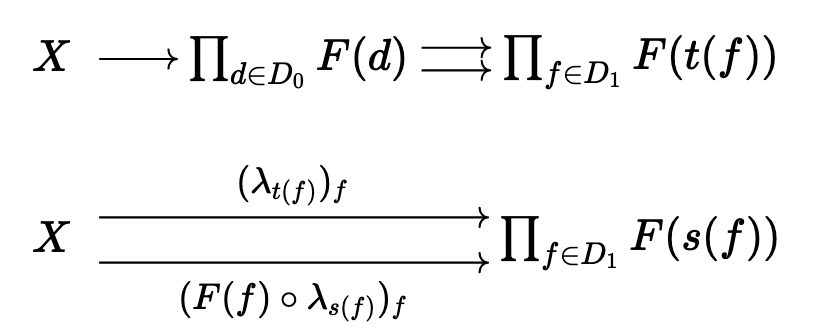
that \(\lim F\) exists, and is the equalizer.
2.3. Abelian Categories
Definition: A category \(C\) is preadditive when it has the structures of abelian groups of \(\Hom_C(-, -)\), such that composition is bilinear; e.g. in torsion free abelian groups, or in \(Ab\) itself. Further, it is additive if it also has finite products and coproducts.
Note that this implies immediately that an additive category has initial and terminal objects.
Lemma: Let \(C\) be an additive cateogry; then for any \(X_1, X_2\), we have \(X_1 \sqcup X_2 \cong X_1 \times X_2\) functorially in \(X_1, X_2\).
Proof: Let us consider
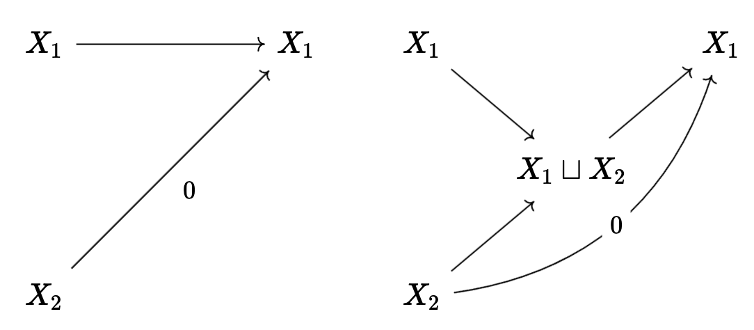
and
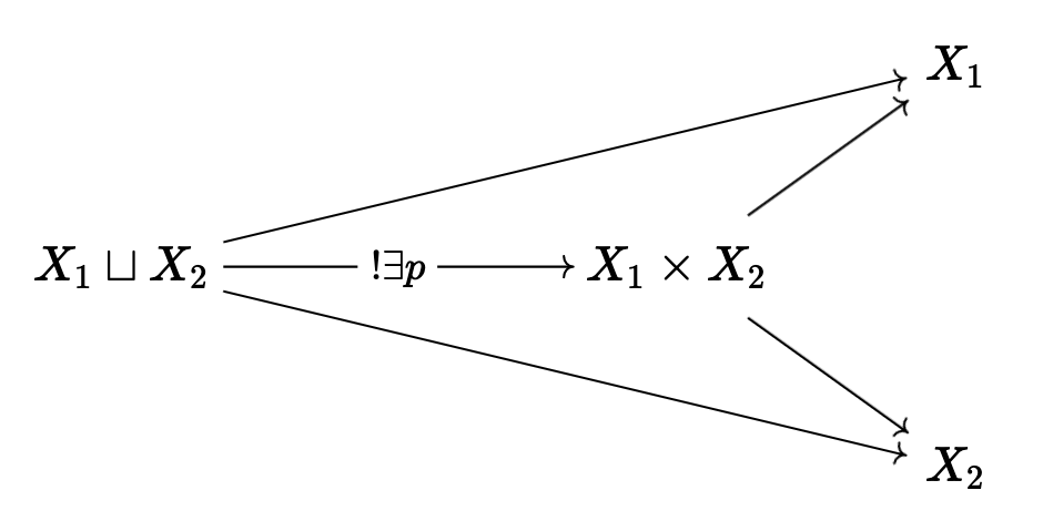
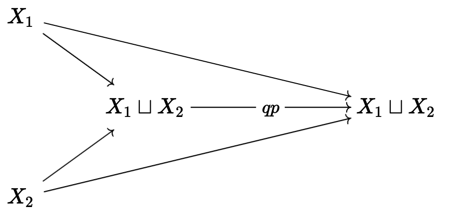
So by reversing arrows we get a map \(q: X_1 \times X_2 \rightarrow X_1 \sqcup X_2\), \(q = \iota_1\pi_1 + \iota_2\pi_2\), where \(\iota, \pi\) are inclusions and projections; then the following diagram can be made to commute:
Definition: The kernel of \(f: X_1 \rightarrow X_2\) in an additive category is the equalizer of \(f_1\) and 0, if it exists; the cokernel is the coequalizer.
Lemma: If \(\iota: K \rightarrow X_1\) is a kernel, then \(\iota\) is a monomorphism.
Definition: An abelian category is an additive category such that all (co)kernels exist (or equivalently, all equalizers and colimits, and therefore the same as all finite limits + colimits), and all epi/monomorphisms are such (co)kernels.
Lemma: If \(A\) is an abelian category amd \(D\) is a small category, then \(\Func(D, A)\) is an abelian category, where the operation is \(F_1 \oplus F_2 = (d \mapsto F_1(d) \oplus F_2(d))\).
Example: \(\Func(FI, Mod_R)\) is an abelian category.
Lemma: Full subcategories of abelian categories are themselves abelian, so long as it contains a zero object, is stable by \(\oplus\), and contains (co)kernels; further, \(B\) preserves (co)kernels.
Disclaimer! We actually need the assumptions; consider \(R = A[x,y]\), and \(A = Mod_R\), and \(B\) the full subcategory of objects \(M\) such that \(M \cong \Ker(M \oplus M \rightarrow M)\), there the first arrow sends \(m \mapsto (mx, my)\) and the second \((a, b) \mapsto am - bm\).
3. Homological Algebra
Definition: A sequence \(X_1 \xrightarrow{f} X_2 \xrightarrow{g} X_3\) is said to be exact (at \(X_2\)) if \(X_1 \rightarrow \Ker(g)\) is an epi.
Definition: We say a functor \(F: A \rightarrow B\) is additive if \(F\) is \(\Z\)-linear on \(\Hom\)-sets and exact if it preserves exact sequences; it also needs to preserve finite products and coproducts, which means that it is equivalent to preserving finite limits and colimits.
Definition: Left/right exact, see Stacks Project Tag 003.
Lemma: If \(F\) is a left adjoint of \(G\), and \(F, G\) are additive, \(F\) commutes with colimits.
Proof: Use Yoneda.
Lemma: Let \(X \in \Ob(A)\), \(A\) an abelian category; then \(\Hom(X, -)\) is a functor \(A \rightarrow Ab\), and it is left exact.
3.1. Projective Modules
Definition: An object \(X\) of \(A\) is said to be projective if \(\Hom(X, -)\) is exact, and dually it is injective if the contravariant Hom is exact. See Stacks Tag 013A for more details.
Lemma: TFAE for \(P \in Mod_R\) projective:
- \(P\) is compact ni \(Mod_R\)
- \(\Hom(P, -)\) commutes with direct sums
- \(P\) is finitely presented
- \(P\) is finitely generated
- \(P\) is a direct summand of a finite free module
Theorem (Quillen): If \(R\) is commutative Noetherian and any projective \(R\)-module is stably free, then the same is true for \(R[t]\).
Theorem (Quillen-Suslind): Any finite projective module over \(k[x_1, \dots, x_n]\) is free (also true over PID).
Lemma: \(k[x]\) is a PID, and for any commutative PID \(R\), TFAE for \(M\) a \(R\)-module:
- \(M\) is a submodule of a free module
- \(M\) is free
- \(M\) is projective
Theorem: Same over local rings, without finiteness conditions.
Proof: See new Matsumura, chapter 2.
Lemma: For \(R\) commutative, TFAE:
- Any stably free \(R\)-module is free
- For all \(m\) and any \(r_1, \dots, r_n\) generating the unit ideal, there is some \(A \in GL_n(R)\) such that \(r_1, \dots, r_n\) form the first column.
For reference, see https://kconrad.math.uconn.edu/blurbs/linmultialg/stablyfree.pdf.
Definition We say that an abelian category \(A\) has enough projectives, if for all \(X \in A\) there is a projective \(P\) which surjects onto \(X\).
For example, \(Mod_R\) certainly has enough injectives, since you can just take a really big free module.
Lemma: Let \(A\) be abelian with small colimits and an object \(P\) which is compact, projective, and a generator; then we have an exact functor \(A \rightarrow Mod_R\), and \(X \mapsto \Hom(P, X)\), where \(R = \End_A(P)\).
Look carefully: this shows that \(Mod_R \cong Mod_{R^{\oplus M}}\) (ref: see Morita equivalence).
3.2. Injective Modules
Definition: \(I \in A\) is injective if \(\Hom(-, I)\) is left exact; similarly, \(A\) has enough injectives if there is always some monic \(X \rightarrow I\) into an injective object.
For modules, see Baer’s criterion, Stacks Tag 05NU.
3.3. Chain Complexes
Definition: \(Ch(A)\), the category of chain complexes of objects of an abelian category \(A\), has objects functors \(\Z \xrightarrow{C_\bullet} A\) \[ \cdots \rightarrow C_{n+1} \xrightarrow{d_n} C_n \xrightarrow{d_{n-1}} C_{n+1} \rightarrow \cdots \] such that \(d_n \circ d_{n+1} = 0\). Furthermore, a morphism of chain complexes is a natural transformation of functors that commutes with the boundary maps. Cochains are chains with the arrows reversed.
Theorem: Let \(A\) abelian and let \(C\) a full subcategory generated by finitely many elements; then there exists a fully faithful functor \(C \rightarrow Mod_R\) for some \(R\).
OK I was sleepy so a topic list: derived categories, derived functors as factoring through the derived category, homotopy, etc.
4. Group Homology
Definition: An abelian group \(A\) is a \(G\)-module if it is a \(\Z[G]\)-module. Note that the category of \(G\)-modules is the same as the functor category from \(G\) to \(Ab\), where the first thing is \(G\) regarded as a groupoid with one element.
Definition: We put: \[ A^G = \{ga = a \mid g \in G, a \in A\} \] and \[ A_G = A / \{ga - a \mid g \in G, a \in A\} \] as functors from \(G\)-mod to \(Ab\).
Lemma: \(A_G \cong \Z \otimes_{\Z[G]}A\), and \(A^G \cong \Hom_G(\Z, A)\), and therefore we have left/right derived functors, which are homology and cohomology functors!
\[ H_0(G, A) = \Z \otimes_{\Z[G]}A = \Z[G]/I_G \otimes{\Z[G]} A = (N\Z[G]) \otimes_{\Z[G]} A \cong NA \] Similar for cohomology.
4.1. Induced Modules
Definition: Let \(H \subset G\), with finite index, and \(M\) an \(H\)-module, and define \[ \Ind^G_H(N) = \Z[H] \otimes_{\Z[H]} M = \{ g \otimes m \mid h \otimes m = 1 \otimes hm \} = \amalg_{s \in G/H} s \otimes M \] and similarly, \[ \Coind^G_H = \Hom_{\Z[H]}(\Z[G], M) = \{f: G \rightarrow M \mid f(hg) = hf(g)\} = \{f(s)\}_{s \in G/H} \] If the index is finite, these are isomorphic.
We define the augmentation ideal to be \(I_G = \Ker(\Z[G] \xrightarrow{\epsilon} \Z)\), under \([g] \mapsto 1\). Then, we know that \(N \rightarrow \Z[G] \rightarrow \Z[G]\) has image \(N \Z[G]\), and kernel \(I_G\). Then, consider that
Lemma: \(\Coind^G_H(-)\) preserves injectives; \(\Ind^G_H(-)\) preserves projectives.
Proof: Use Tensor-Hom adjunction.
Lemma: For \(H \subset G\), \(M\) an \(H\)-module, then there are canonical isomorphisms \[ H^r(G, \Coind^G_H M) \cong H_r(G, M) \] \[ H_r(G, \Ind^G_H M) \cong H_r(G, M) \]
Proof: Take injective/projective resolutions of \(M\), and take coinduced/induced modules.
Definition: We have two different restrictions, which take \(M \rightarrow \Coind^G_HM\) (where \(m \mapsto (g \mapsto gm\)) or \(M \rightarrow \Ind^G_HM\) (where, under \([G:H] < \infty\), sends \(m \mapsto \sum_{s \in G/H}s \otimes s^{-1}m\)), and two different corestrictions, which take \(\Coind^G_HM \rightarrow M\) (where, under \([G:H] < \infty\), sends \(\varphi^H \mapsto \sum_{s \in G/H}s \varphi(s^{-1})\)) and \(\Ind^G_HM \rightarrow M\) (where \(g \otimes m \mapsto gm\)).
Now consider the following,
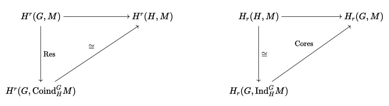
and the opposite maps, as above.
Lemma: If \([G:H] = r < \infty\) then the composition \(\text{Cores} \circ \text{Res}\) is just multiplication by \(r\).
Proof: Check in degree 0, and then it follows for (co)homology.
Theorem: Assume that \(G\) is finite, with order \(m\); further, suppose we have \(m: A \rightarrow A\) is an isomorphism. Then, all higher (co)homology groups vanish, and if \(N = \sum_{g \in G}[g]\), then \(H_0(G,A) = H^0(G,A) = NA\).
Proof: Take \(H\) trivial and call it a day.
4.2. Explicit Resolutions
We want to just take a resolution of \(\Z\) that will let us compute arbitrary homology/cohomology. We take \[ \cdots \rightarrow \Z[G \times G \times G] \xrightarrow{\delta} \Z[G \times G] \xrightarrow{\delta} \Z[G] \xrightarrow{\epsilon} \Z \rightarrow 0 \] where \[ \delta([g_0, \dots, g_r]) = \sum_{i=0}^r(-1)^i[g_0, \dots, \widehat{g_i}, \dots, g_r] \] Then, I claim that once we apply \(\Hom(-, M)\), we get \[ \cdots \rightarrow \Hom_G(\Z[G^{n-1}], M) \rightarrow \Hom_G(\Z[G^n], M) \rightarrow \Hom_G(\Z[G^{n+1}], M) \rightarrow \cdots \] and this sequence will have the cohomology we want. In particular, note that these \(\Hom\) groups are just all map \(G^r \rightarrow M\), which we willl call \(C^r(G, M)\).
5. Simplicial Sets
Definition: Let \(\Delta\) be the category of nonempty finite totally ordered sets with nondecreasing maps as morphisms.
Definition: Let \(C\) be a category, and \(Simp(C)\) of \(C\) simplicial objects is the functor category \(\Func(\Delta^{op}, C)\), and \(Cosimp(C)\) is \(\Func(\Delta, C)\).
Example: Let \(C = Top\), so that \(\Delta^n = \Delta([m]) = \{f: [m] \rightarrow \R_+ \mid \sum_{i=0}^mf(i) = 1\}\). Then, let \(\alpha: [n] \rightarrow [m]\), and set \[ \Delta(\alpha)(f) = \left(j \in [m] \mapsto \sum_{i \in \alpha^{-1}(j)}f(i)\right) \] So we obtain \(\Delta^\bullet \in Cosimp(Top)\).
Definition: The singular simplicial set \(S(X)\) attached ti \(X \in Top\) is defined as \[ S(X) = \Hom_{Top}(\Delta^\bullet, \underline{X}) \in Simp(Set) \]
Lemma: \(X \mapsto S(X)\) has a left adjoint, denoted \(E \mapsto | E|\), the “geometric realization.”
Proof: Note that \(\Hom_{Simp(Sets)}(E, S(X))\) is just the collection of (continuous) maps \(f: E_n \rightarrow \Hom_{Top}(\Delta^n, X)\) satisfying the appropriate naturality condition, but this is again just the maps \(f: E_n \times \Delta^n \rightarrow X\), again satisfying the appropriate naturality condition; but lastly, this must be all maps \(f: \bigsqcup_{n \in \N}E_n \times \Delta^n \rightarrow X\) satisfying that \(\forall x \in E_n\) and \(\forall s \in \Delta^m\) and \(\forall \alpha : [m] \rightarrow [n]\), we have that \(f(E(\alpha)x, s) = f(x, \Delta(\alpha)s)\).
But since \(|E| = \bigsqcup_{n \in \N}E_n \times \Delta^n / \sim\), where \(\sim\) is generated by \((E(\alpha)x, s) \sim (x, \Delta(\alpha)s)\), these are exactly the same.
Theorem: For \(X \in Top\), TFAE:
- \(X\) is homotopically equivalent to some \(|E|\)
- The adjunction \(|S(X)| \rightarrow X\) is a homotopy equivalence
- \(X\) is Hausdorff and there is some partition \(X = \bigsqcup_n \bigsqcup_{i \in C_n} X_i\) into subsets, such that
- A subset \(F \subset X\) is closed iff \(\forall i, F \cap \overline{X_i}\) is closed in \(\overline{X_i}\).
- \(\forall i \in C_n\), there is a \(\Delta^n \xrightarrow{f} X\) continuous such that \(f|_{(\Delta^n)^\circ}\) is a homomorphism onto \(X_i\), and \(f({\delta \Delta^n}) \subset\) a finite union of all cells of degree \(< n\).
And if any of the above hold, then \(X\) is a CW complex.
Theorem: There is a notion of homotopy for simplicial sets, such that it is equivalent to the homotopy category of CW complexes, where one map is given by \(| \cdot |\) and the other by \(S(\cdot)\).
Under the idea of simplicial sets, we have that
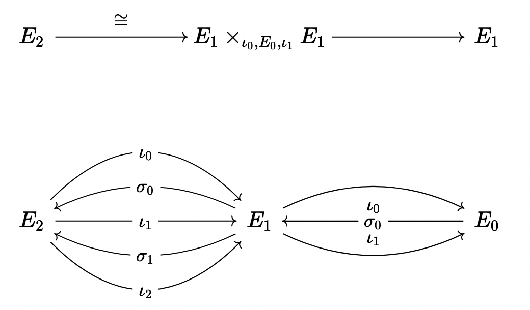
actually represents a category, with \(E_1\) maps, \(E_0\) objects, and \(E_2\) composition! And \(n\) categories are just tacking on \(E_3, \dots, E_n\) onto this diagram!
5.1. Classifying Spaces
Let \(S\) be a nonempty set, and \(\underline{S}_n\) the maps \([n] \rightarrow S\), which is now a simplicial set. But its geometric realization is homotopic to a point, so it is not that interesting; but if we consider \(G\) a group, then \(\underline{G}\) has a right \(G\) action, which takes \(fg \mapsto (x \mapsto f(x)g\).
Definition: We set \(BG = \underline{G}/G\) to be the classifying space of \(G\).
Definition: Let \(A\) be an abelian category, and let \(X \in Simp(A)\); we construct \(C(X) \in Ch(A)\), by setting \(C(X)_n = X_n\), and letting the differential map be \(\sum_{j=0}^n(-1)^j\iota_j^{*}\) where \(\iota_j: [n - 1] \rightarrow [n]\) is an injection missing \(j\).
Definition: For \(A\) abelian, we may now define \(H_n(X)\) to be the homology of the chain \(H_n(C(X))\).
Definition: We have another complex, the Moore complex, while will be in degree \(n\) \[ N(X)_n = \cap_{j=0}^{n-1} \Ker(\iota_j^*: X_n \rightarrow X_{m-1}) \subset C(X)_n, \ \ \delta_n = (-1)^n \iota_n^* \]
Lemma: The inclusion \(N(X) \rightarrow C(X)\) induces \(H_n(N(X)) \cong H_n(X)\).
Theorem (Dold-Kan Correspondence): The functor \(Simp(A) \xrightarrow{N} Ch_{\geq 0}(A) \) is an equivalence of abelian categories.
Definition: We set for \(X \in Simp(Sets)\), \(H_n(X, R) = H_n(R^{\oplus X})\), and if \(X \in Top\), then \(H_n(X, R) = H_n(S(X), R)\), where the homology is taken with coefficients in \(R\), a ring.
Theorem: The inclusions \(\lambda_0, \lambda_1: X \rightarrow X[0, 1]\), given by \(\lambda_i: x \mapsto (x, i)\) induce the same homomorphism \(H_n(X, R) \rightarrow H_n(X \times [0, 1], R)\).
Corollary: If \(f, g: X \rightarrow Y\) are homotopic, then \(H_n(f, R) = H_n(g, R)\); further, if \(f: X \rightarrow Y\) is a homotopy equivlance then \(H_n(f, R)\) is ana isomorphism.
Proof: There is some \(H: X \times [0, 1] \rightarrow Y\) which is a homotopy between \(f,g\). Then,
\begin{align*} H_n(f) = H_n(\lambda_0)H_n(H) = H_n(\lambda_1)H_n(H) = H_n(g) \end{align*}Theorem:
- If \(X \in Simp(Set)\), then \(X \rightarrow S(|X|)\) ia a homotopy equivalence, and in particular \(H_n(X, R) \cong H_n(S(|X|), R)\).
- If \(X\) is a CW complex, then \(H_n(|S(X)|, R) \cong H_n(X, R)\).
Example: Let us consider \(S^1\). In particular, \(S^1\) is a line with endpoints identified, so we may let
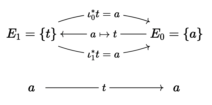
Then, \(E_n\) is just generated by formally adding degeneracies of \(t\); let us look at \(C(R[E])\), so we have a complex \[ 0 \rightarrow R[t] \xrightarrow{t \mapsto \iota_0^*t - \iota_1^*t = 0} R[a] \rightarrow 0 \] so we see that \(H_1(S^1, R) \cong H_0(S^1, R) \cong R\). If we don’t glue things together, so it’s just an interval \(I\), then we get the complex \[ 0 \rightarrow R[t] \rightarrow R[a_0] \oplus R[a_1] \rightarrow 0 \] so we see that \(H_1(I, R) = 0\), \(H_0(I, R) = R\).
We may also do \(S^1 \times S^1\), under the triangulation
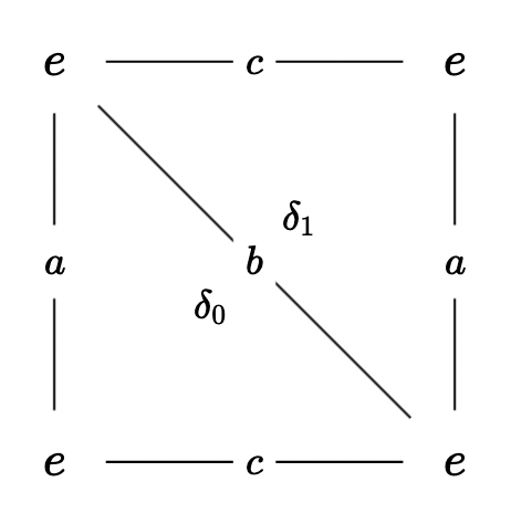
so we can see the complex will be \[ R[\delta_0] \oplus R[\delta_1] \rightarrow R[a] \oplus R[b] \oplus R[c] \rightarrow R[e] \rightarrow 0 \] so that \(H_0 = R, H_1 = R^{\oplus 2}, H_2 = R\).
In general, if \(X \in Top\), then \(C(S(X), R)\) will end in \[ \text{free modules on paths} \rightarrow \text{free modules on points} \rightarrow 0 \] so it must be \(H_0\) is the set of free \(R\)-modules on \(X / (f(0) \sim f(\lambda), f \in C^0([0, 1], X))\), or the set of path-connected components of \(X\).
Theorem: \(H_1(X, \Z) \cong \pi_1(X)^{ab}\).
Proof: \(\pi_1\) is just the homotopy classes of \(f: \Delta^1 \rightarrow X\), such that \(f\iota_0 = f\iota_1\); in particular, we have a map \(\pi_1 \rightarrow Z_1(C(S(X)))\), where \(f \mapsto [f]\), where we have that \(df = [f\iota_0] - [f\iota_1] = 0\).
Then, we have, since \(Z_1(C(S(X))) / B_1 \cong H_1\) is abelian, we have a map that factors \(\pi_1^{ab} \rightarrow H_1\). Then, just check injective/surjective.
Theorem: Let \(G\) be a group; then the \(H_n(G, R) \cong H_n(BG, R) \cong H_n(|BG|, R)\). In fact, \(\pi_1(BG) = G, \pi_k(BG) = 0\) otherwise; that is, it is a \(K(G,1)\) space.
5.2. Homotopy Groups
Let \(X\) be a topological space, and set \(\pi_k(X)\) the fundamental group in degree \(k\), e.g. all maps \(S^k \rightarrow X\) identified up to homotopy. Note that in general, \(\pi_0\) is just a set, \(\pi_1\) is a group, and \(\pi_k\) is an abelian group for higher \(k\).
Theorem: The group homology of \(G\) is the same as the singular homology of a \(K(G, 1)\) space.
We will also take \[ \Conf_n(\C) = \{(z_1, \dots, z_n) \in \C^n \mid z_i \neq z_j \text{ for } i \neq j\} \] and show that it is path connected and has \(\pi_1\) the pure braid group.
Definition: A continuous map \(p: E \rightarrow B\) is a fiber bundle with typical fiber \(F\) if \(\forall b \in B\), there is \(U\) open containing \(b\) such that
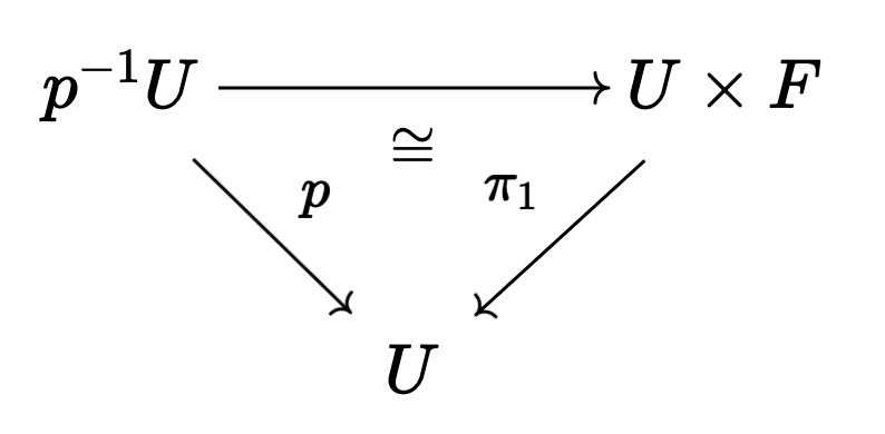
conmmutes.
Note that if \(p: E \rightarrow B\) is a fibration with fiber \(F\) path-connected, we can make a long exact sequence \[ \cdots \rightarrow \pi_2 (B) \rightarrow \pi_1 (F) \rightarrow \pi_1 (E) \rightarrow \pi_1 (B) \rightarrow 0 \]
Theorem: \(\pi_1(\Conf_n(\C))\) is the pure braid group, and every other homotopy class is trivial.
Let \(O_n = \Conf_n(\C_n)\) be the covering space of \(U_n\) so that it is a fiber bundle with fiber \(S_n\). In this case, we have a s.e.s. \[ 1 \rightarrow \pi_1 (O_n) \rightarrow \pi_1 (U_n) \rightarrow S_n \rightarrow 1 \]
Proof: Consider \(n = 2\); then, \(\C^2\setminus \Delta \cong S^1\), so \(\pi_1(O_2) \cong \pi_1 (S^1) \cong \Z\). Then, \(U_2 = \{(s_1, s_2) \mid s_1^2 \neq s_2\}\). Then we see that \[ U_2 \rightarrow \C^2 \setminus \C \times \{0\} \cong S^1 \] and the s.e.s. must be \[ 0 \rightarrow \Z \rightarrow \Z \rightarrow \Z/2 \rightarrow 0 \]
If you think a little, then \(\pi_1(U_n)\) must be the (geometric) braid group, and \(\pi_1(O_n)\) must be the (geometric) pure braid group; in fact we will take this by fiat and make this our definitions for these groups.
Furthermore, the higher homotopy groups must be 0, since we have that \(O_n \rightarrow O_{n-1}\) via forgetting the last coordinate has fiber \(\C \setminus \{z_1, \dots, z_{n-1}\}\), and so we must have that for \(k \geq 2\), we have the l.e.s. \[ \cdots \rightarrow \pi_k (F) = 0 \rightarrow \pi_k(O_n) \rightarrow \pi_k (O_{n-1}) = 0 \rightarrow \cdots \]
The last thing to do is to check that our geometric groups line up with the group representations \[ \widetilde{B}_n \cong \left\langle (\sigma_i)^{n-1}_{i=1} \mid \sigma_i\sigma_j = \sigma_i\sigma_i \text{ for } |i - j| > 2, \sigma_i\sigma_j\sigma_i = \sigma_j\sigma_i\sigma_j \text{ for } |i - j| = 1\right\rangle \] The entire thing is kind of long and annoying! So I will just make the remark that it’s really clear if you take \(\sigma_i\) to be the braid that crosses the threads connecting \(i\) and \(i + 1\) once. In fact, it is good enough to check the pure braid group lines up with the representation (I am not typing this)
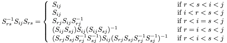
But we can just check this for \(S_{ij}\) to be (draw a picture, and don’t look at this!) \[ S_{ij} = \sigma_{j-1}^{-1}\sigma_{j-2}^{-1}\cdots\sigma_{i+1}^{-1}\sigma_{i^2}\sigma_{i+1}\cdots\sigma_{j-2}\sigma_{j-1} \] for \(i < j\).
6. Spectral Sequences
If we have some s.e.s. \[ 1 \rightarrow G \rightarrow G' \rightarrow G'' \rightarrow 1 \] how do we relate \(H_p(G')\) and \(H_p(G'', H_q(G))\)?
Let \(F: A \rightarrow B\) a left exact functor between abelian categories with enough injectives; and \(G: B \rightarrow C\) also left exact. For \(X \in \Ob(A)\), we want to compute \(R(G \circ F)(X)\), the right dervied functor of the compositions; in particular if we take an injective resultion \(X \rightarrow I^\bullet\), then \(R(G \circ F)(X)\) is quasiisomorphic to \((G \circ F)(I^\bullet)\), and \(RF(X)\) is quasiisomorphic to \(F(I^\bullet)\).
Lemma: If \(0 \rightarrow X \rightarrow Y \rightarrow Z \rightarrow 0\) in \(B\) and if \(X \rightarrow I^\bullet_X, Z \rightarrow I^\bullet_Z\) are injective resolutions, then there is an exact sequence \[ 0 \rightarrow I_X^\bullet \rightarrow I_Y^\bullet \rightarrow I_Z^\bullet \rightarrow 0 \] and we may write \(Y \rightarrow I_Y^\bullet\) an injective resolution.
Lemma (Cartan-Eilenberg Resolution): Let \(B\) be an abelian category with enough injectives, and \(C^\bullet\) a bounded below complex. Then, there is a sequence such that
- For all \(q\), \[ C^{q} \rightarrow I^{q,0} \rightarrow I^{q,1} \] is an injective resolution.
- For all \(q\), \[ Z^q(C^\bullet) \rightarrow Z^q(I^{\bullet, c}) \rightarrow Z^q(I^{\bullet, I}) \] is an injective resolution.
- Same for \(B^q = \Im(d^{q-1}) \subset Z^q\)
- Same for \(H^q\)
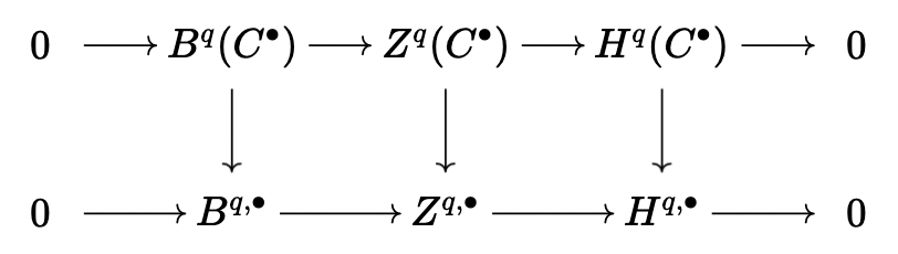
Proof: Take s.e.s. \[ 0 \rightarrow B^q(C^\bullet) \rightarrow Z^q(C^\bullet) \rightarrow H^q(C^\bullet) \rightarrow 0 \] and \[ 0 \rightarrow Z^q(C^\bullet) \rightarrow C^q \rightarrow B^{q+1}(C^\bullet) \rightarrow 0 \] Now let \(H^{q, \bullet}\) be an injective resolution of \(H^q(C^\bullet)\), and \(B^{q, \bullet}\) be an injective resolution of \(B^q(C^\bullet)\). From the earlier lemma, let \(Z^{q, \bullet}\) be an injective resolution of \(Z^{q}(C^\bullet)\) fitting into a diagram
Again by the lemma, there is an injective resolution \(C^q \rightarrow I^{q, \bullet}\) fitting into the diagram
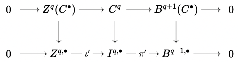
We have \(C^\bullet \rightarrow I^\bullet\) by construction, and we define a differential \(I^{q, \bullet} \rightarrow I^{q+1,\bullet}\) as the composition given by \(\iota' \circ \iota \circ \pi'\), where \(\iota: B^{q+1, \bullet} \rightarrow Z^{q+1, \bullet}\) is the inclusion.
Then, we have \[ \Ker(d^q) \cong Z^{q,\bullet}, \ \Im(d^q) \cong B^{q+1, \bullet} \] which gives use everything we want. See Stacks Tag 015G for more details.
Now, let \(A \xrightarrow{F} B \xrightarrow{G} \rightarrow C\) and \(X \rightarrow I^\bullet\) be as earlier (we technically need \(B\) with small coproducts), and let \(F(I^\bullet) \rightarrow I^{\bullet, \bullet}\) be a Cartan-Eilenberg resolution.
Definition: We put \[ \Tot^n(I^{\bullet,\bullet}) = \bigoplus_{p+q = n}I^{p,q} \] with differential \(d: \Tot^m \rightarrow \Tot^{m+1}\), given by \(d^{n}|_{I^{p,q}} = d_{\uparrow} + (-1)^p()d_{\rightarrow}\).
We have \(F(I^q) \xrightarrow{\iota} I^{0, q} \subset Tot^q(I^{\bullet, \bullet})\); similarly, let \(x \in F(I^q)\); then we have \[ d^q_{\Tot}\iota x = d_{\uparrow}\iota x + d_{\rightarrow}^0 \iota x = d_{\uparrow} \iota x = \iota \delta^q x \]
We have a few questions:
- Is \(F(I^\bullet) \rightarrow \Tot^\bullet(I^{\bullet,\bullet})\) is a quasiisomorphism? If so, then \(RGRF X^\bullet\) is quasiisomorphic to \(\Tot^\bullet(G(I^{\bullet, \bullet})\).
- How do we compute the cohomology of \(\Tot^\bullet\)?
We can do this more generally.
Definition: A filtered complex is a complex \(D^\bullet\) alongside \(\Fil^q(D^\bullet)\), such that
- \(\Fil^q(D^\bullet) \hookrightarrow D^\bullet\) is an inclusion of a subcomplex.
- We have \(\Fil^q(D^\bullet) \hookleftarrow \Fil^{q+1}(D^\bullet)\).
- \[ \bigcup_q \Fil^q(D^\bullet) = D^\bullet \]
- \[ \bigcap_q \Fil^q(D^\bullet) = 0^\bullet \]
In particular, notice that the complex \(D^\bullet = \Tot^\bullet(I^{\bullet, \bullet})\) is equipped with a filtration \[ \Fil^q(I^n) = \bigoplus_{p' + q' = n, q' \geq q}I^{p', q'} \] and we note that \(\Fil^q / \Fil^{q+1} \cong I^{n-q, q}\). Similarly, we have the analogy that \(I^{p,q}\) should be \[ \Gr^q (D^{p+q}) = \Fil^q (D^{p+q}) / \Fil^{q+1}(D^{p+q}) \]
We want to understand the cohomology of a filtered complex \(D^\bullet\) in terms of \(\Gr^q(D^\bullet)\). Let’s work in a module category for now.
Warning! Indicies are probably wrong. Check them!
We have then that \[ H^q(C^\bullet) = \frac{\{x \in C^q \mid dx = 0\}}{\{dy \mid y \in C^{q-1}\}} \] as well as \[ \{x \in C^q \mid dx = 0\} = \bigcap_{r \geq 0} \{ x \in \Fil^p(C^q) \mid dx \in \Fil^{p+r}(C^q)\} = \bigcap_{r \geq 0}F_{r}^{p,q} \] and \[ \{dy \mid y \in C^{q-1}\} = \bigcup_{r \geq 0} \{ y \in \Fil^{p-r}(C^q) \mid dy \in \Fil^{p}(C^q)\} \] Now let \[ Z_{r}^{p,q} = \frac{F^{p,q}_r}{F^{P+1,q-1}_{r-1}} \] and \[ B^{p,q}_r = \frac{d F^{p+1-r,q+r-2}_{r-1} + \Fil^{p+1}C^{p+q}}{d \Fil^{p+1}(C^{p+q})} = \frac{dF_{r-1}^{p+1-r, q+n-2}}{dF_r^{p+1-r, q+r-2}} \]
Let us finally define \[ E_r^{p,q} = \frac{Z_r^{p,q}}{B^{p,q}_n} \] But now, we have a mapping \[ F_r^{p,q} \xrightarrow{d} F_r^{p+r,q+1-r} \] so we have, for example,
\begin{align*} E_0^{p,q} &= \Gr^p(C^{p+q}) = I^{p,q} \\ E_1^{p,q} &= \frac{\Ker(\Gr^p(C^{p+1}) \rightarrow \Gr^{p+1}(C^{p+q}))}{d \Gr^{p}(C^{p+q-1})} = H^{p+q}(\Gr^p(C^\bullet)) \\ \end{align*}and so on.
We examine the differential more closely now; in particular we have a map \(F_n^{p,q} \xrightarrow{d_n} E^{p+r, q+1-r}_r\), sending \([x] \mapsto [dx]\). Cruicially, this is well-defined (check!) and factors through \(Z_n^{p,q}\); if \(x \in F_{r-1}^{p+1,q-1}\) we have \(x \in F^{p+r+1-r,q+1-r+r-2}_{r-1}\), hence \([dx] \in B_r^{p+r, q+1-r}\) which is killed in the quotient. And so it must factor through \(E_r^{p,q}\) as well, since \(d^2 = 0\).
Definition: We call \(E_r^{p,q}\) the \(r^{th}\) page of the spectral sequence associated to the origiinal filtered complex.
Theorem: We have a natural isomorphism \[ E_{r+1}^{p,q} \cong \frac{\Ker(d_2: E_r^{p,q} \rightarrow E_{r}^{p+r,q-r+1})}{\Im(d_r: E_r^{p-r,q+r-1} \rightarrow E_r^{p,q})} \] given just by inclusion; we may call this map \(\iota\). In other words, we go to the next page of the spectral sequence by taking (co)homology.
Proof: Let \(x \in F_r^{p,q}\) with \(dx = 0\) in \(E_r^{p+r,q+1-r}\); thus \(dx = dy + z\) for \(y \in F_{r-1}^{p+1,q-1}\) and \(z \in F_{r-1}^{p+r+1, q-r}\). Thus, \(d(x-y) = z\), so \([x] = [x-y] \in Z_n^{p,q}\); thus \(x - y \in F_{n+1}^{p,q}\), and \([x] = \iota [x-y]\). So the
So \(\iota\) is surjective; to check injectivity, let \(x \in F_{r+1}^{p,q}\) such that \(\iota [x] = 0\), i.e. such that \([x] = [dy]\) in \(E_{r}^{p,q}\), where \(y \in F_r^{p-r, q+r-1}\). Thus, we have \(x - dy = dz + t\), where \(z \in F_{r-1}^{p+1-r, q+r-2}\) and \(t \in F_{r-1}^{p+1,q-1}\), so \(x = d(y+z) + t\). Now note that \(dt = dx \in \Fil^{p+r+1}(C^{p+q+1})\), so it must be that \(t \in F_r^{p+1,q-1}\) in fact. So we win, since \(d(y+z) = x-t \implies y + z \in F_{r}^{p-r, q+r-1}\), and we conclude that \([x] = 0\).
Definition: We say that the spectral sequence degenerates on page \(r\), if for all \(r' \geq r\), we have that \(d_{r'} = 0\).
Prop: If \(E_r^{p,q}\) degenerates at \(r\), the filtration on \(H^\bullet(C)\) indueced by \(H^n(\Fil^p)\) has \(p^{th}\) graded terms isomorphic to \(E_r^{p, n-p}\), and we put \(E_n^{p,q} \implies H^{p,q}(C)\).
Example: We take the following diagram, where the rows are exact and the left and right columns are exact.

We may take the spectral sequence with \(0^{th}\) page \(d_{ \rightarrow }\), and we obtain by exactness \(E_1^{p,q} = 0\); so it stabilizes at \(r = 1\), so \(H^n(\Tot) = 0\). However, if we take the spectral sequence with \(0^{th}\) page \(d_{\uparrow}\), we have that the \(E_1\) page looks like this
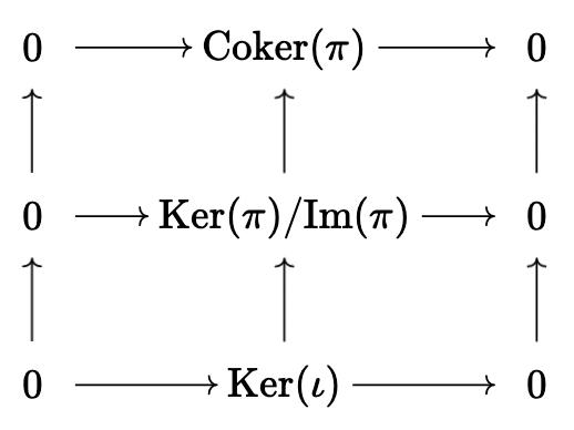
but since either the target or the source of each morphism is 0, we see that the sequence degenerates. So it must be that \(H^1(\Tot) = \Ker(\iota) = 0\), \(H^2(\Tot) = \frac{\Ker(\pi)}{\Im(\iota)} = 0\), and \(H^3(\Tot) = \text{Coker}(\pi) = 0\). This proves the Nine Lemma.
6.1. Grothendieck Spectral Sequences
Theorem: Let \(F: A \rightarrow B\) be left exact between abelian categories with enough injectives, and let \(G: B \rightarrow C\) be left exact, such that for all injective \(I \in \Ob(A)\), \(F(I)\) is \(G\)-acyclic; that is, \(R^qG(F(I)) = 0\) for \(q > 0\). Then, there is a natural exact sequence such that \[ E^{p,q}_2 = R^pG(R^qFX) \implies R^{p+q}(G \circ F)(X) \] for \(X \in \Ob(A)\). In particular, we have that \(R(GF)(X)\) is quasiisomorphic to \(RG \circ RF (X)\).
Proof: Let \(X \rightarrow I^\bullet\) be an injective resolution, and let \(F(I^\bullet) \rightarrow I^{\bullet, \bullet}\) be a Cartan-Eilenberg Resolution. Then, there is an induced homomorphism \(F(I^\bullet) \rightarrow \Tot(I^{\bullet, \bullet})\) of complexes, and it is a quasiisomorphism.
To see this, we note that by construction, \[ E^{p,q}_{1,\rightarrow} = \begin{cases} F(I^q) & p = 0 \\ 0 & p \neq 0 \end{cases} \] so it must be that this spectral sequence degenerates at the \(E_1\) page, so \(F(I^q) \cong H^q(\Tot(I^{\bullet, \bullet}))\). We apply \(G(I^{\bullet, \bullet})\), and see that
\begin{align*} E^{p,q}_{1, \rightarrow} &= R^qG(F(I^q)) \\ E^{p,q}_{1, \uparrow} &= G(H^{p,q}) \end{align*}since the sequences \[ 0 \rightarrow B^{p-1,q} \rightarrow Z^{p,q} \rightarrow H^{p,q} \rightarrow 0 \] and \[ 0 \rightarrow Z^{p,q} \rightarrow I^{p,q} \rightarrow B^{p+1,q} \rightarrow 0 \] split since everything in sight is injective, so they remain exact after applying \(G\). Then, we have that \((H^{p,q})_{p \in \Z}\) is an injective resolution of \(H^{p}(F(I^\bullet)) = R^pF(X)\). Therefore, we have that \(E_{2, \uparrow}^{p,q} = R^qG(R^pFX)\). Furthermore, since \(\Tot^\bullet(G(I^{\bullet, \bullet})) = G(\Tot^\bullet(I{^\bullet,\bullet}))\), and since from before \(\Tot^\bullet(I^{\bullet, \bullet})\) is quasiisomorphic to \(F(I^\bullet)\), we must have \[ \Tot\bullet(I^{\bullet, \bullet}) \cong RG(F(I^\bullet)) \cong RG \circ RF(X) \]
Now note that by assumption \(R^qG(F(I^q)) = 0\) for \(q > 0\), so then \[ E^{p,q}_{1, \rightarrow} = \begin{cases} GF(I^p) & q = 0 \\ 0 & q \neq 0 \end{cases} \] Thus we have that this spectral sequence degenerates at \(E_1\), and thus \(GF(I^\bullet)\) is quasiisomorphic to \(\Tot(G(I^{\bullet,\bullet}))\).
6.2. Application to Group Homology
Let \(G\) be a group, and \(H^q(G, -)\) the right derived functor of the left exact functor \(Mod_{R[G]} \rightarrow Mod_R\) sending \(M \mapsto M^G\), and \(H_q(G, -)\) the left dervied functors of \(M \mapsto M_G\).
Let us consider an exact sequence \[ 1 \rightarrow P \rightarrow G \rightarrow Q \rightarrow 1 \] Then for \(M\) a \(G\)-module, we have that \(M^G = (M^P)^Q\), i.e. we have
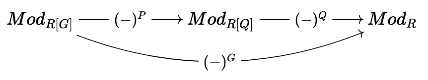
Then, if \((-)^P\) sends \(R[G]\)-injectives to \(H^\bullet_r(P, -)\) acyclic then we obtain a natural spectral sequence \[ E_2^{p,q} = H^q(Q, H^p(P, M)) \implies H^{p+q}(G, M) \]
Lemma (Five-term exact sequence): Let \(M^{p,q}\) be a double complex in the first quadrant, \(A\) its total complex, and \(E^{p,q}_2 \implies H^n(A)\) be the second page of its spectral sequence. Then there is an exact sequence \[ 0 \rightarrow E_2^{1,0} \rightarrow H^1(A) \rightarrow E_2^{0,1} \rightarrow E_2^{2,0} \rightarrow H^2(A) \]
7. Symmetry Groups
Look at the following table of homology:
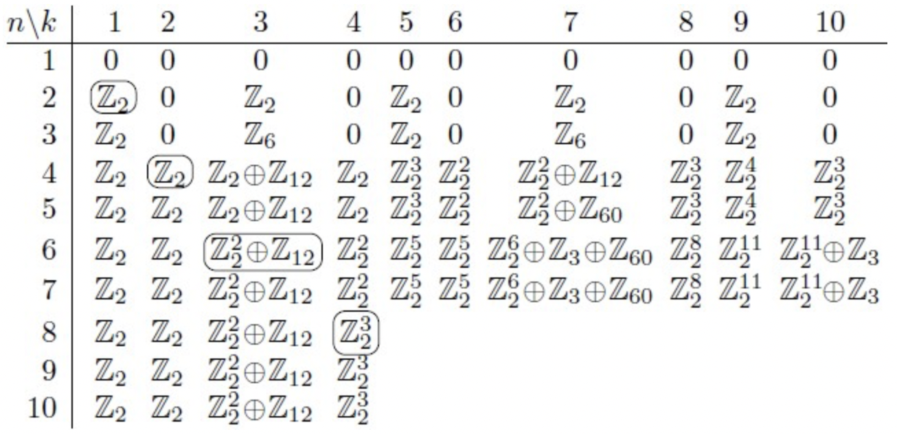
Then we have a few conjectures:
- \(\forall n \geq 2q\), \(H_qS_n \rightarrow H_qS_{n+1}\) is an isomorphism
- \(\forall n\), \(H_qS_{n-1} \rightarrow H_qS_n\) is an injection
- \(\forall n\), \(H_qS_n / H_qS_{n-1}\) is killed by \(n\).
The last one is actually easy to prove; just use restriction/corestriction.
Remember the ealier discussion of contravariant functors \(FI \rightarrow Sets\).
Let \(W_p = C_\bullet (\Hom_{FI}(-, [1, p])) \in Ch(Mod_{\Z[S_p]})\).
Theorem: \(H_0W_p \cong \Z\). Furthermore, if \(0 < q < p/2\), we have \(H_qW_p = 0\).
The strategy goes as follows: let \(P_\bullet\) be a projective resolution of \(\Z\) as an \(\Z[S_n]\) module (for example, the bar complex is a free resolution). Then, we look at the double complex \(E^{0}_{p,q} = P_p \otimes_{\Z[S_n]} (W_n)_q\). Then, we see that
- \(E^{1,\uparrow}_{p,q} = H_p(S_n, (W_n)_q)\)
- \(E^{1,\rightarrow}_{p,q} = P \otimes H_qW_n\)
- \(E^{2, \rightarrow}_{p,q} = H_p(S_n, H_qW_n)\)
Then, use the last theorem and look at the \(E^{2}\) page and win.
Let us examine \((W_n)_q\) as a \(\Z[S_n]\) module more closely. In particular, we have that \((W_n)_q \cong \Z[\Hom([q], [1,n])]\), so if \(p \leq q\), it is \(0\), and if \(p \geq q +1\), we have that it must be \[ \bigoplus_{f \in \Hom([q, [1,n]]) / S_n}\Z[S_n / \{\sigma \in S_n \mid \sigma|_{\Im(f)} = \id\}] \] Note that the summand is also just \(\Ind^{S_n}_{S_{n-p-1}} \Z\). But by Schapiro’s lemma, we see that \[ H_p(S_n, (W_n)_q) \cong \bigoplus_{f \in \Hom([p],[1,n]) / S_n} H_p(S_{n-q-1}, \Z) \]
Note that we have the differential mapping \[ d[f] = \sum_{i=0}^q(-1)^i[f \circ e_i] \] where each \(e_j\) is a non-decreasing injection that misses \(j\).
We can endow \(W_n\) with the increasing filtration \[ \Fil_p W_n = \begin{cases} W_p & p \leq n \\ W_n & p > n \end{cases} \] with graded parts \[ (\Gr_p W_n)_q = \begin{cases} 0 & p > n \text{ or p < 0 } \\ \bigoplus_{\substack{f: [q] \rightarrow [1,p] \\ p-1 \in \Im(f)}} & \Z[f] \end{cases} \] We may also rewrite this to be \[ (\Gr_p W_n)_q = \bigoplus_{j=0}^q D_j(W_{p-1})_{q-1} \] where \[ D_j[f] = \left[ i \mapsto \begin{cases} f(i) & i < j \\ p & i = j \\ f(i-1) & i > j\end{cases} \right] \]
But does this preserve the differential? We compute that
\begin{align*} dD_j[f] &= \sum_{i=0}^q(-1)^i(D_j[f])e_i \\ &= \sum_{i=0}^{j-1} (-1)^i(D_{j-1}[f \circ e_i]) + \sum_{i=j+1}^{q} (-1)^i(D_{j}[f \circ e_{i-1}])\\ &= \sum_{0 \leq i < j}(-1)^uD_{j-1}([f \circ e_i]) - \sum_{j \leq i \leq q - 1}(-1)^{i}D_j([f \circ e_i]) \end{align*}Note that since \(f\) misses \(p\), the \(i=j\) term vanishes. So unfortunately the \(D_j\) symbols don’t form a subcomplex. But we do have that \(dD_0[f] = - D_0d[f]\)! And everything gets messy afterwards pretty quickly. Further, we do have that for all \(k\), \(\bigoplus_{j \leq k}D_jW_{p-1}\) is a subcomplex of \(\Gr_pW_n\).
We can also talk about the homology of \(W_n\). In particular, we see that
\begin{align*} W_0 &= 0 \\ W_1 &= \Z[0] \\ W_2 &= [\Z[\id] \oplus \Z[\tau] \rightarrow \Z[i_0] \oplus \Z[\iota_1]] \\ H_0W_2 &= \Z^{\oplus 2}/\Z(-1, 1) \cong \Z \\ H_1W_2 &= \Z([\id] + [\tau]) \cong \Z \end{align*}And so on.
Now, note the spectral sequence associated to the filtration, which is
\begin{align*} E_{p,q}^0 &= (\Gr_pW_n)_{p+q} \\ E_{p,q}^{1} &= H_{p+q}(\Gr_p W_n) \\ \end{align*}We still need to compute the second page.
We consider the filtration \[ \widetilde{\Fil}_k(\Gr_pW_n) = \bigoplus_{i \leq k}(\Gr_p W_n)_{q+1}e_i \] with graded parts \[ \widetilde{\Gr}_j(\Gr_pW_n) \cong W_{p-1}[1] \] noting that \(W_{p-1}[1]\) (the shifted complex) is the same as \((W_{p-1})_{q-1}\) in degree \(q\), with a negative differential. We should have \(H_0 \cong \Z\), \(H_i \cong 0\) for \(i \neq 0, p-1\), and \(H_{p-1}\) is something probably nonzero. Then, in particular we see that the spectral sequence degenerates at the \(E_2\) page.
And then you do some stuff; I was sick, so forgive me for missing the rest.
8. \(FI\)-Modules
Again, let \(FI\) be the category of finite sets with injective maps. First, we fix a ring \(k\), and let a \(FI\)-module (over \(k\)) be a functor \(FI \rightarrow Mod_k\). For example, we may take \[ F^{(d)}: S \mapsto k[\Hom_{FI}(d, S)] \] In particular, we have for \(V\) any \(FI\)-module, we have that \[ \Hom_{Mod_{FI}}(F^{(d)}, V) = \Hom(\Hom_{FI}(d, -), V) = V_d \] In particular, any \(FI\)-module is a quotient of a direct sum of copies of \(F^{(d)}\): if \(M_d \rightarrow V_d\) is surjective with \(M_d\) free, then \[ \bigoplus_{d \geq 0} M_d \otimes_k F^{(d)} \rightarrow V \] is surjective.
Definition: A \(FI\)-module \(V\) is a finitely generated (in degrees \(\leq D\)) if for all \(d \leq D\), \(V_d\) is a finitely generated \(k\)-module, and if \[ \bigoplus_{d \leq D}V_d \otimes_k F^{(d)} \rightarrow V \] is surjective.
Theorem: If \(k\) is Noetherian commutative, then the category of finitely generated \(FI\)-modules over \(k\) is Noetherian.
For \(\lambda\) = \((\lambda_j)_j\) with \(\lambda_j \geq \lambda_{j+1}\), we may define \[ V_n(\lambda) = \begin{cases} V_{(n - \sum \lambda_j, \lambda_1, \lambda_2, \dots)} & n \geq \lambda_1 + \sum_{j \geq 1} \lambda_j \\ 0 & \text{otherwise} \end{cases} \] For example, we see that \(V_n(0)\) is the trivial representation of \(k\), \(V_n(1)\) is the standard representation, and so on. (In this case we need \(k\) a field.)
Prop: There is a f.g. \(FI\)-module \(V_\bullet(\lambda)\) such that in degree \(d\) it is simply \(V_d(\lambda)\).
Proof: Take \[ V(\lambda)_d = \colim_{T} k[S_d]c_T \] where the colimit is in the category with objects Young tabelaus and the indexing set is tabelaus with shape \((d - |\lambda|, \lambda)\).
Theorem: Let \(k\) be a field of characteristic \(0\). Then, a \(FI\)-module \(W\) is finitely generated if and only if
- For all \(d \rightarrow d+1\), the induced map \(W_d \rightarrow W_{d+1} = \text{Res}^{G_{d+1}}_{G_d}W_{d+1}\) is (eventually) injective.
- For all \(d \rightarrow d+1\), the induced map \(\text{Ind}^{G_{d+1}}_{G_d}W_d \rightarrow W_{d+1}\) is (eventually) surjective.
- \(c_{\lambda, n}\), a multiple of \(W_n(\lambda)\) in \(W_n\) is independent of \(n\) for \(n > N\) (uniform representation stability).
When combined with the Noetherianity conditions, it becomes really easy to show representational stability!
Proof: We start with the easier direction, which is \(\impliedby\). Let \(N\) such that for all \(d \geq N\), \(k[S_{d+1}] \otimes_{k[S_d]} W_d \rightarrow W_{d+1}\) is surjective. Then, \(k[S_{d}] \otimes_{k[S_N]} W_N \rightarrow W_{d+1}\). Thus \(F^{(N)} \otimes W_N \rightarrow W\) is surjective in degree \(\geq N\), and so \(W\) is f.g. in degree \(\leq N\).
To do the other direction, we need more setup.
Definition: The injectivity degree (resp. surjectivity degree) is the smallest \(s \geq 0\) (if it exists), such that \((W_n)_{S_{n-r}} \rightarrow (W_{n+1})_{S_{n+1-r}}\) is injective (resp. surjective) for \(n \geq s + r\).
Lemma: If \(V \rightarrow W\) is surjective, then the surjectivity degree of \(W\) is at most the surjectivity degree of \(V\). The opposite result holds for the injectivity degree.
Lemma: The \(FI\)-module \(F^{(d)} = k[\Hom_{FI}(d, -)]\) has injectivity degree 0 and surjectivity degree \(d\).
Now let \(W\) be a finitely generated \(FI\)-module in degree \(\leq N\); let \(F\) be a finite direct sum of \(F^{(d)}\) with \(d \leq N\) such that \(F \rightarrow W\) is a surjection; we have that \(\text{surj deg}(W) \leq \text{surj deg}(F) \leq N\).
Let \[ 0 \rightarrow K \rightarrow F \rightarrow W \rightarrow 0 \] be exact; then \(K\) is a submodule of \(F\) and is thus finitely generated. Then, in particular we have from the snake lemma in the diagram
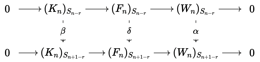
that \(\text{inj deg}(W) \leq \text{inj deg}(K) \leq M\).
Prop: Let \(W\) be a \(FI\)-module over \(k\) with characteristic \(0\); then \((W_n)_n\) is uniformly representation stable with stable range \(n \geq \max\{\text{inj deg}(W) , \text{surj deg}(W) \} + \text{weight}(W)\), where \[ \text{weight}(V) = \max \{ |\lambda| \mid V_n(\lambda) \text { appears in some } W_n\} \]
Theorem: The \(FI\)-module \(n \mapsto H^q(P_n, \Q)\) is uniformly representation stable for \(n \geq 4q\).
In particular, we may compute that \[ H^1(P_n, \Q) \cong V_n(0) \oplus V_n(1) \oplus V_n(2) \] for \(n \geq 4\) and \[ H^2(P_n, \Q) \cong V_n(1)^{\oplus 2} \oplus V_n(1, 1)^{\oplus 2} \oplus V_n(2)^{\oplus 2} \oplus V(2, 1)^{\oplus 2} \oplus V(3) \oplus V(3, 1) \] for \(n \geq 7\) (so the bound is not always sharp).
It remains to prove the noetherianity proposition. In spirit, it will be similar to the Hilbert basis thoerem.
Consider now the category of \(FI-Mod_R\); if \(W\) is such a \(FI\)-module, consider the grading of \(W\) given by \[ R(W) = \bigoplus_{n \geq 0} (W_n)_{S_n} \] where \((W_n)_{S_n} \xrightarrow{T} (W_{n+1})_{S_{n+1}}\), where \(T\) is induced by the cannonical injection. In particular, we already require \(R\) to be a \(\Q\)-algebra since we need left exactness of coinvariants. If \(W \subset F^{(d)}\), then \(R(W) \subset R(F^{(d)})\); then, \(R(W)\) is f.g. as a \(R[T]\) module. Next, we also have that \[ W_n \cong \bigoplus_{\lambda}(W_n \otimes V_n(\lambda)^*) \otimes V_n(\lambda) \]
Then, if \(W \subset F^{(d)}\), then we have a bound \(m\), namely the weight and each \(R(W \otimes V(\lambda))\) is finitely generated; hence, \(W\) is finitely generated. \[ \]
Prop: Let \(R\) be noetherian, \(W)\) a sub \(FI-Mod_R\) of \(F^{(d)}\). Then \(W\) is f.g.
Proof: Recall that \[ F^{(d)} = S \mapsto R[\Hom_{FI}(d, S)] \] We may induct on \(d)\), starting with \(d = -1\), \(F^{(-1)} = 0\); as mimick the proof of the Hilbert basis theorem.
Let \(A\) be a finite set; we consider the shift \[ W[A]: S \in FI \mapsto W_{S \sqcup A} \]
In particular, we can map \((F^d[A])_s \rightarrow (F^{(d)})_s\) surjectively, just by taking \[ [f: d \rightarrow S \sqcup A] \mapsto \begin{cases} [f] & \Im(f) \subset S \\ 0 & \text{otherwise} \end{cases} \] and so we discover a s.e.s \[ 0 \rightarrow \bigoplus_{\substack{A' \subset A \\ A' \neq \emptyset \\ \text{bij } d\setminus (d - |A'|) \rightarrow A'}} (F^{d-|A'|})_s\rightarrow (F^d[A])_s \rightarrow (F^{(d)})_s \rightarrow 0 \] Correspondingly, \[ 0 \rightarrow K \cap W[A] \rightarrow W[A] \rightarrow W^{(A)} \rightarrow 0 \] By induction, \(K \cap W[A]\) is finitely generated, and \(W\) is finitely generated \(\iff W[a]\) is finitely generated, and we can prove that \(W^{(A)}\) is finitely generated. (Skipped)
Theorem: Fix \(R\) nootherian, and let \(N \subset M\) \(FI\)-modules, with \(M\) f.g. Then \(N\) is f.g. as well.
Proof: Induct on the number of nonzero graded pieces in \(M\).
Theorem: Let \(k\) be a field, and let \(W\) be a f.g. \(FI-Mod_R\); then \(\dim_k(W_n)\) is eventually polynomial in \(n\).